The Developer’s Guide to Quantum Noise and Error Mitigation in Qiskit

Table of Contents

Introduction

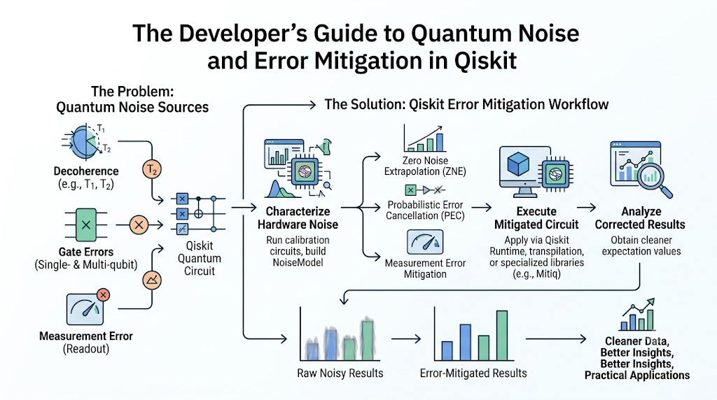
Quantum computing represents a fundamental shift in how we process information. By harnessing the principles of quantum mechanics—such as superposition, interference, and entanglement—quantum processors can tackle complex mathematical problems that are practically intractable for classical supercomputers. In today’s NISQ (Noisy Intermediate-Scale Quantum) era, quantum hardware consists of tens to hundreds of physical qubits that remain highly sensitive to their surrounding environment. Until full Fault-Tolerant Quantum Computing (FTQC) becomes a reality, researchers and software engineers rely on error mitigation techniques to extract accurate expectation values from noisy quantum circuits. This comprehensive guide breaks down what quantum noise is, why it occurs, how common error types manifest, how error mitigation differs from full quantum error correction, and how you can write noise-resilient quantum programs using modern frameworks like Qiskit.

What is Quantum Noise?

In classical computing, information is processed using transistors that hold binary states: 0 or 1. These states are robust, voltage-backed physical representations that can maintain their values reliably for years.

In quantum computing, the fundamental unit of information is the qubit (quantum bit). A qubit can exist in a state of 0, 1, or any continuous linear combination (superposition) of both:

$$\vert{}\psi\rangle = \alpha\vert{}0\rangle + \beta\vert{}1\rangle$$

Here, $\alpha$ and $\beta$ are complex probability amplitudes. Because these quantum states are delicate wave functions, even minute interactions with external energy or matter can alter their fragile phase and probability distributions.

Quantum noise refers to any unwanted environmental disturbance, physical imperfection, or operational inaccuracy that alters the quantum state of a qubit away from its intended trajectory during a computation.

Classical Bit State:    [0]  or  [1]     --->  Extremely stable against environment
Quantum Qubit State:   |ψ⟩ = α|0⟩ + β|1⟩  --->  Delicate state disrupted by heat, stray electromagnetic fields, or cross-talk

Why Noise is a Fundamental Challenge in Quantum Computing

Noise is not merely a software bug; it is a physical barrier rooted in the laws of quantum thermodynamics. Unlike classical bits—which benefit from high signal-to-noise margins—qubits must remain isolated from their environment to preserve their quantum behavior, yet coupled to external controls so developers can manipulate them using quantum gates.

This creates the quantum control paradox:

To keep a quantum state pure, you must isolate the qubits completely from thermal, magnetic, and radiation influences.
To perform a computation, you must interact with the qubits using microwaves, lasers, or magnetic fields.

Every control pulse introduced to perform a quantum operation inevitably opens a channel for unwanted environmental energy to leak in. As quantum circuits grow deeper (more sequential operations) and wider (more entangled qubits), accumulative noise destroys fragile quantum information before the calculation finishes.

Understanding Qubits and Decoherence

To grasp how noise degrades a computation, it helps to understand how a qubit’s state decays over time. The loss of a qubit’s quantum properties due to environmental interaction is broadly termed decoherence.

Decoherence is characterized by two primary physical relaxation times:

                          ┌──────────────────────────┐
                          │    Quantum Noise Types   │
                          └────────────┬─────────────┘
                                       │
                ┌──────────────────────┴──────────────────────┐
                ▼                                             ▼
     ┌──────────────────────┐                      ┌──────────────────────┐
     │  Energy Relaxation   │                      │ Dephasing / Phase    │
     │      Time (T1)       │                      │     Relaxation (T2)  │
     ├──────────────────────┤                      ├──────────────────────┤
     │ Qubit decays from    │                      │ Loss of phase angle  │
     │ |1⟩ state down to    │                      │ relationship         │
     │ ground state |0⟩.    │                      │ in superposition.    │
     └──────────────────────┘                      └──────────────────────┘

$T_1$ Energy Relaxation Time (Thermal Relaxation): The time it takes for an excited qubit state ($\vert{}1\rangle$) to lose energy to its environment and decay back to its ground state ($\vert{}0\rangle$). This acts similarly to a battery losing its charge over time.
$T_2$ Dephasing Time (Phase Coherence Time): The duration over which the relative phase angle between $\vert{}0\rangle$ and $\vert{}1\rangle$ in a superposition state remains predictable. Fluctuating magnetic fields cause the quantum phase to randomize without necessarily changing the qubit’s energy level.

Because $T_2$ is always less than or equal to $2T_1$, a quantum circuit must finish executing all gate operations well within the $T_2$ window. If a circuit’s runtime exceeds $T_2$, the quantum system loses its superposition characteristics and devolves into a random classical mixture.

Common Sources of Quantum Noise

Quantum noise originates from multiple physical layer vulnerabilities across different quantum hardware platforms (e.g., superconducting circuits, trapped ions, neutral atoms, or photonic systems):

Thermal Fluctuations: Tiny amounts of ambient heat cause unwanted energy transitions in superconducting qubits, forcing them out of ground states.
Control Signal Imperfection: Microwave or laser pulses used to drive quantum gates may suffer from power drifting, phase jitter, or timing calibration offsets.
Cross-talk: Applying a gate to one physical qubit can inadvertently apply weak stray fields to neighboring qubits on the chip.
Stray Electromagnetic Fields: Fluctuations in earth’s magnetic fields, ambient radio frequencies, or cosmic rays interfere with energy levels.
Impurity Scattering: Defects in physical materials (such as oxide layers in Josephson junctions) create charge noise that destabilizes qubit frequencies.

Types of Quantum Errors

Mathematically, quantum noise transforms ideal quantum states via quantum error channels. The primary quantum errors encountered during execution include:

                              ┌──────────────────────────┐
                              │   Types of Quantum       │
                              │         Errors           │
                              └────────────┬─────────────┘
                                           │
         ┌──────────────────┬──────────────┴───────────────┬──────────────────┐
         ▼                  ▼                             ▼                  ▼
  ┌──────────────┐   ┌──────────────┐              ┌──────────────┐   ┌──────────────┐
  │   Bit Flip   │   │  Phase Flip  │              │ Gate Errors  │   │ Measurement  │
  │  (X Error)   │   │  (Z Error)   │              │  (Coherent)  │   │ (SPAM Error) │
  └──────────────┘   └──────────────┘              └──────────────┘   └──────────────┘

1. Bit Flip Error ($X$ Error)

A bit flip converts a $\vert{}0\rangle$ state into a $\vert{}1\rangle$ state or vice-versa. It acts like an unintended Pauli-$X$ gate applied to the qubit:

$$X\vert{}0\rangle = \vert{}1\rangle, \quad X\vert{}1\rangle = \vert{}0\rangle$$

2. Phase Flip Error ($Z$ Error)

A phase flip leaves the energy populations untouched but flips the relative phase sign of the superposition state. It acts like an unintended Pauli-$Z$ gate:

$$Z\left(\frac{\vert{}0\rangle + \vert{}1\rangle}{\sqrt{2}}\right) = \frac{\vert{}0\rangle – \vert{}1\rangle}{\sqrt{2}}$$

3. Combined Bit and Phase Flip ($Y$ Error)

A simultaneous bit and phase error represented mathematically by the Pauli-$Y$ matrix ($Y = iXZ$).

4. Gate Errors & Depolarizing Noise

Gate errors occur during operation. Single-qubit gates often have high fidelity (e.g., $>99.9\%$), but entangling two-qubit gates (like CNOT or CZ) have higher error rates (often $0.1\%$ to $2\%$). Depolarizing noise models an operation where, with a probability $p$, the qubit state is completely randomized into an isotropic mixture.

5. Measurement & SPAM Errors

SPAM stands for State Preparation And Measurement. Measurement errors occur when a qubit in state $\vert{}0\rangle$ is misread as $1$, or a qubit in state $\vert{}1\rangle$ is misread as $0$ by the readout electronics during final signal acquisition.

NISQ (Noisy Intermediate-Scale Quantum) Devices Explained

Coined by physicist John Preskill in 2018, the term NISQ (Noisy Intermediate-Scale Quantum) defines our current era of quantum computing:

Intermediate-Scale: Quantum processors contain anywhere from 50 to a few thousand physical qubits.
Noisy: Qubits are uncorrected and susceptible to environmental interference, restricting circuit execution depth to a limited number of gate steps.

In NISQ devices, individual qubits are used directly as operational units without the massive redundancy overhead required for fault tolerance. Consequently, running complex quantum algorithms (like Shor’s factoring algorithm or deep Quantum Phase Estimation) directly on raw NISQ hardware results in noise dominating the output signal.

However, NISQ hardware remains extremely valuable for executing hybrid quantum-classical algorithms—such as the Variational Quantum Eigensolver (VQE) and the Quantum Approximate Optimization Algorithm (QAOA)—when paired with algorithmic noise reduction.

Quantum Error Mitigation vs Quantum Error Correction

A critical distinction in quantum information science is the difference between quantum error mitigation (QEM) and quantum error correction (QEC). While both strategies aim to solve hardware noise, they operate on different principles and target different computational phases.

  ┌─────────────────────────────────────────────────────────────────────────┐
  │                      Quantum Noise Strategy Map                         │
  ├────────────────────────────────────┬────────────────────────────────────┤
  │    Quantum Error Mitigation (QEM)  │   Quantum Error Correction (QEC)   │
  ├────────────────────────────────────┼────────────────────────────────────┤
  │ • Target: Near-Term NISQ Devices   │ • Target: Future Fault-Tolerant    │
  │ • Uses statistical post-processing │ • Uses active real-time feedback   │
  │ • Zero physical qubit overhead     │ • High physical qubit overhead     │
  │ • Estimates Expectation Values ⟨O⟩ │ • Preserves arbitrary Qubit States │
  └────────────────────────────────────┴────────────────────────────────────┘

Key Differences Comparison Table

Feature	Quantum Error Mitigation (QEM)	Quantum Error Correction (QEC)
Primary Goal	Reduces noise effects statistically in post-processing.	Eliminates hardware errors continuously during runtime.
Qubit Overhead	Low to zero additional physical qubits needed.	High overhead (requires 100s to 1,000s of physical qubits per logical qubit).
Sampling Overhead	Scales exponentially with circuit depth/noise level.	Constant or polynomial runtime scaling once active.
Target Output	Expectation values ($\langle O \rangle$) of quantum observables.	Arbitrary, state-preserved logical quantum outcomes ($\vert{}\psi\rangle$).
Hardware Era	NISQ Era (Available and used today).	Fault-Tolerant Era (Future production systems).
Feedback Loop	Classical post-processing of repeated measurements.	Real-time active quantum non-demolition error syndrome measurement.

Popular Error Mitigation Techniques

Modern error mitigation relies on mathematical techniques to infer what an ideal, noise-free result would look like based on data gathered from noisy runs.

                  ┌───────────────────────────────────────────────┐
                  │      Popular Error Mitigation Protocols       │
                  └───────────────────────┬───────────────────────┘
                                          │
       ┌──────────────────────────────────┼──────────────────────────────────┐
       ▼                                  ▼                                  ▼
┌──────────────────────────────┐ ┌──────────────────────────────┐ ┌──────────────────────────────┐
│  Zero Noise Extrapolation    │ │ Probabilistic Error          │ │ Measurement Error            │
│  (ZNE)                       │ │ Cancellation (PEC)           │ │ Mitigation (M3 / TREX)       │
├──────────────────────────────┤ ├──────────────────────────────┤ ├──────────────────────────────┤
│ Intentionally scales noise   │ │ Inverts learned noise        │ │ Characterizes and inverts    │
│ up (λ=1, 2, 3) and fits curve│ │ channels using probabilistic │ │ classical assignment readout │
│ back to zero noise (λ=0).    │ │ circuit combinations.        │ │ matrices.                    │
└──────────────────────────────┘ └──────────────────────────────┘ └──────────────────────────────┘

1. Zero Noise Extrapolation (ZNE)

Zero Noise Extrapolation (ZNE) intentionally amplifies noise in a controlled manner.

How it works: The algorithm executes a quantum circuit at the hardware’s base noise level ($\lambda = 1$), and then runs modified versions with artificially scaled noise factors (e.g., $\lambda = 2, 3, 5$).
Noise Scaling Methods: Noise is typically scaled by replacing single gates with identity pairs (e.g., replacing CNOT with CNOT-CNOT-CNOT) or stretching pulse lengths.
Extrapolation: A curve (linear, polynomial, or exponential) is fitted to the measured expectation values across these noise levels. Extrapolating the curve back to zero noise ($\lambda = 0$) provides an estimate of the noise-free value.

2. Probabilistic Error Cancellation (PEC)

Probabilistic Error Cancellation (PEC) provides an unbiased estimate of quantum expectation values.

How it works: PEC models noisy hardware gates as linear combinations of ideal operations. By sampling a collection of noisy circuits according to a calculated quasi-probability distribution and weighting the outputs, noise channels can be inverted mathematically.
Trade-off: While PEC yields unbiased expectation estimates, sampling overhead grows exponentially with circuit depth, requiring more shots.

3. Readout / Measurement Error Mitigation (M3 & TREX)

Readout errors occur when a state is measured incorrectly.

Matrix-Free Measurement Mitigation (M3): Computes readout corrections efficiently for large qubit registers without constructing massive full-assignment matrices.
Twirled Readout Error Extinction (TREX): Applies random Pauli-X gates immediately prior to measurement (twirling) to symmetrize and eliminate readout bias.

4. Symmetry Verification & Post-Selection

Many physical systems respect conservation laws (such as particle number or total spin symmetry). If a quantum circuit simulation violates known physical symmetries upon final measurement, those corrupted samples can be filtered out during post-processing.

How Error Mitigation Works in Practice

Executing an error-mitigated quantum workload follows a distinct workflow between classical control computers and physical quantum processors:

┌─────────────────────────────────────────────────────────────────────────────┐
│                       Error Mitigation Execution Loop                       │
└─────────────────────────────────────────────────────────────────────────────┘

  1. Circuit Formulation      2. Noise Characterization     3. Circuit Variant
     & Compilation               & Scaling                     Execution
   ┌──────────────────┐        ┌──────────────────┐        ┌──────────────────┐
   │ Define Quantum   │        │ Learn hardware   │        │ Run original and │
   │ Circuit & Target │ ─────► │ error rates &    │ ─────► │ scaled circuits  │
   │ Observable       │        │ calibrate models │        │ on hardware      │
   └──────────────────┘        └──────────────────┘        └────────┬─────────┘
                                                                    │
  5. Mitigated Result         4. Statistical Extrapolation          │
     Output                      & Post-Processing                  │
   ┌──────────────────┐        ┌──────────────────┐                 │
   │ Noise-Mitigated  │ ◄───── │ Fit data models  │ ◄───────────────┘
   │ Expectation      │        │ & apply inversion│
   │ Value ⟨O⟩        │        │ matrices         │
   └──────────────────┘        └──────────────────┘

Circuit Formulation: Define your target quantum circuit and the observable quantities (such as Pauli-Z operator expectation values) you wish to evaluate.
Noise Characterization: Run diagnostic routines (like Randomized Benchmarking) to measure device noise rates.
Variant Execution: Generate circuit variants (e.g., scaled circuits for ZNE or twirled circuits for PEC) and execute them across thousands of measurement shots on real hardware.
Statistical Processing: Aggregate expectation outcomes and apply mathematical transformations (extrapolation, inversion matrices, or symmetry filtering).
Mitigated Output: Produce an accurate expectation value estimate that reflects the true underlying physics far better than raw hardware runs.

Error Mitigation in Qiskit and Other Quantum Frameworks

Modern open-source frameworks like Qiskit make error mitigation accessible to developers without requiring them to write low-level pulse protocols from scratch.

Simulating Noise and Applying Mitigation in Qiskit

Below is an example showing how to build a noisy circuit simulation using qiskit_aer and explore depolarizing noise models.

Python

# Import core Qiskit and Qiskit Aer components
import numpy as np
from qiskit import QuantumCircuit
from qiskit_aer import AerSimulator
from qiskit_aer.noise import NoiseModel, depolarizing_error

# Step 1: Create a 2-qubit Bell State circuit
qc = QuantumCircuit(2)
qc.h(0)
qc.cx(0, 1)
qc.measure_all()

# Step 2: Build a custom synthetic noise model
noise_model = NoiseModel()

# Define a 1-qubit gate error (0.5% error) and 2-qubit gate error (3% error)
error_1qubit = depolarizing_error(0.005, 1)
error_2qubit = depolarizing_error(0.03, 2)

# Add errors to specific gate operations
noise_model.add_all_qubit_quantum_error(error_1qubit, ['h'])
noise_model.add_all_qubit_quantum_error(error_2qubit, ['cx'])

# Step 3: Instantiate noisy simulator backend
noisy_sim = AerSimulator(noise_model=noise_model)

# Step 4: Run the noisy simulation
job = noisy_sim.run(qc, shots=2000)
result = job.result()
counts = result.get_counts()

print("Noisy Execution Results (Bell State):")
print(counts)
# Output will show expected |00> and |11> states along with noise counts (|01>, |10>)

In production settings using IBM Quantum hardware, higher-level Qiskit Runtime primitives (Sampler and Estimator) expose built-in resilience settings. Setting resilience_level=1 applies readout mitigation, resilience_level=2 applies Zero Noise Extrapolation (ZNE), and resilience_level=3 employs advanced techniques like Probabilistic Error Cancellation (PEC).

Challenges and Limitations of Error Mitigation

While error mitigation has unlocked quantum utility—allowing 100+ qubit systems to perform calculations that rival classical approximations—it is not a permanent replacement for fault tolerance:

Exponential Sampling Overhead: As circuit depth or qubit count increases, methods like ZNE and PEC require exponentially more sample shots to maintain statistical precision.
Expectation Value Restriction: Most error mitigation techniques only correct expected averages ($\langle O \rangle$) over many runs. They cannot output an uncorrupted single-shot quantum state, which is required for algorithms like Grover’s Search or Shor’s Algorithm.
Assumptions About Noise: Many mitigation routines assume noise is uncorrelated or Markovian. Highly coherent, non-Markovian, or drifting noise profiles can reduce the accuracy of extrapolation models.

Real-World Applications and Research Examples

Error mitigation techniques are already powering discovery across academic and industrial research labs:

Quantum Chemistry & Material Science: Researchers use error-mitigated VQE algorithms on superconducting processors to calculate the ground state energy levels of complex molecules, such as iron-sulfur clusters and lithium hydride, with chemical-grade accuracy.
Condensed Matter Physics: High-depth simulations of 2D transverse-field Ising models use Zero Noise Extrapolation to observe magnetic phase transitions and quantum chaos dynamics on real quantum hardware.
Financial Optimization: Portfolio optimization algorithms running QAOA rely on measurement error mitigation (M3) to prevent misreading optimal weight configurations in dense solution spaces.

Best Practices for Writing Noise-Resilient Quantum Programs

To get the cleanest results from today’s quantum computers, developers should follow these engineering best practices:

┌─────────────────────────────────────────────────────────────────────────────┐
│                    Noise-Resilient Programming Checklist                    │
├─────────────────────────────────────────────────────────────────────────────┤
│ 1. Transpile for Hardware Topology: Minimize CNOT depth & swap gates.       │
│ 2. Apply Dynamical Decoupling (DD): Insert pulse sequences during idles.    │
│ 3. Enable Readout Mitigation: Correct measurement bias systematically.       │
│ 4. Leverage Native Gate Sets: Avoid unnecessary gate conversions.           │
│ 5. Enforce Symmetry Constraints: Filter out non-physical outputs.           │
└─────────────────────────────────────────────────────────────────────────────┘

Optimize Circuit Depth: Always transpile your circuit to match the target device’s native gate set and coupling map to eliminate unnecessary SWAP gates.
Use Dynamical Decoupling (DD): Insert sequences of fast pulses (e.g., $X-X$ sequences) on idling qubits during long gate delays to prevent dephasing.
Calibrate Gate Routing: Select physical qubits with the highest current $T_1/T_2$ times and lowest two-qubit error rates using real-time backend status data.
Integrate Symmetry Filtering: Post-select results by discarding outputs that violate problem-specific conservation rules (e.g., total electron count in chemistry models).

Future of Fault-Tolerant Quantum Computing

The ultimate goal of the field remains Fault-Tolerant Quantum Computing (FTQC).

To reach FTQC, multiple physical qubits are combined using surface codes, color codes, or LDPC (Low-Density Parity-Check) codes to form a single logical qubit. Logical qubits detect and correct physical errors in real-time faster than they propagate, protecting the computation indefinitely.

Today (NISQ Era):              Physical Qubit  --->  Noisy / Short-lived
                               
Future (Fault-Tolerant Era):   [ Physical Qubit x1,000 ]  --->  1 Logical Qubit
                                 (With Active Error Correction)    (Protected)

Error mitigation serves as the crucial bridge. It enables practical quantum utility on NISQ machines today while quantum hardware engineers work toward building physical systems with the higher qubit counts needed for full quantum error correction.

Career Opportunities in Quantum Computing Research

The demand for professionals who understand quantum noise and mitigation is growing rapidly across both industry and academia.

Key Roles

Quantum Error Correction Scientist: Designs and proves mathematical thresholds for topological codes and FTQC architectures.
Quantum Software Engineer: Builds open-source tools, compilers, and transpiler passes for noise-aware execution.
Quantum Control Engineer: Develops low-level microwave pulse calibration routines to minimize physical gate error channels.
Quantum Applications Researcher: Applies error-mitigated NISQ algorithms to practical problems in chemistry, finance, and machine learning.

Frequently Asked Questions

What is quantum noise in simple terms?

Quantum noise refers to unwanted environmental disturbances—such as heat, stray magnetic fields, or control signal imperfections—that disrupt sensitive quantum states in a quantum processor.

Why can’t we just insulate quantum computers from all noise?

While quantum processors are cooled to near absolute zero in dilution refrigerators, they must still connect to external control lines to perform computations. These control channels inevitably introduce noise.

What is the difference between decoherence and relaxation?

Decoherence is the overall decay of quantum behavior. Energy relaxation ($T_1$) specifically refers to a qubit losing energy and decaying from state $\vert{}1\rangle$ to $\vert{}0\rangle$, while dephasing ($T_2$) refers to the loss of phase alignment in a superposition state.

Is quantum noise the same as a software bug?

No. A software bug is an error in code logic. Quantum noise is physical interference caused by environmental interactions and hardware imperfections during computation.

What is Zero Noise Extrapolation (ZNE)?

ZNE is an error mitigation strategy where a circuit is run at intentionally increased noise levels. A mathematical curve is fitted to the outputs to extrapolate what the result would be at zero noise.

Can error mitigation fix every quantum computation?

No. Error mitigation requires extra classical sampling runs, which grow exponentially with circuit size. It is effective for moderate circuit depths but cannot scale indefinitely like full quantum error correction.

How many physical qubits are needed to make one logical qubit?

Depending on error rates and code architecture (such as surface codes), it typically takes anywhere from hundreds to thousands of physical qubits to construct a single fault-tolerant logical qubit.

What tools can I use to practice error mitigation in Python?

You can use frameworks like Qiskit (with Qiskit Aer noise models and Qiskit Runtime Primitives) or open-source libraries like Mitiq.

What is a SPAM error?

SPAM stands for State Preparation And Measurement error. It represents inaccuracies that occur during initial qubit setup or during final measurement readout.

When will full Fault-Tolerant Quantum Computing arrive?

While roadmaps vary across industry leaders, multi-logical-qubit systems and fault-tolerant architectures are actively being developed, with commercial fault-tolerant computing expected to emerge over the next decade.

Conclusion

Quantum noise is one of the most important challenges in modern physics and computer science. While environmental interaction and decoherence limit what current NISQ systems can achieve on their own, quantum error mitigation provides a powerful way to extract reliable, accurate results from noisy hardware today. By combining hardware improvements with techniques like Zero Noise Extrapolation, Probabilistic Error Cancellation, and symmetry filtering, the community is pushing near-term systems to their limits. Mastering these concepts is essential for anyone building a career in quantum software development, algorithm design, or quantum research.