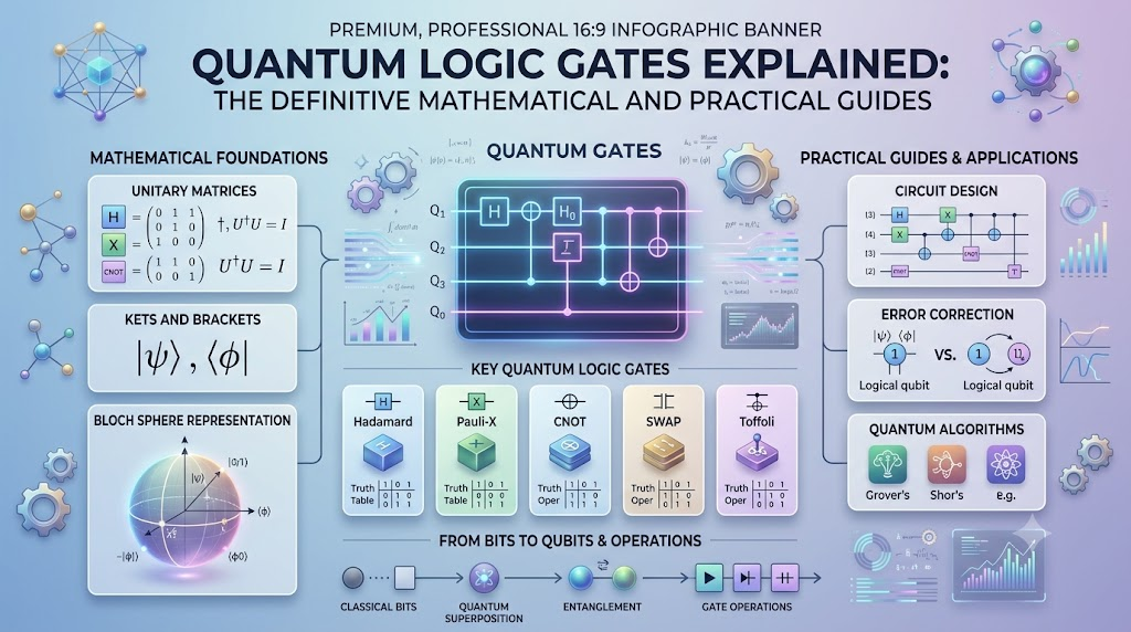
Classical computing is built on switches that are definitively either on or off, represented as a 0 or a 1. Quantum computing departs from this binary constraint. By using the physical principles of superposition and entanglement, quantum processors run algorithms capable of evaluating complex computational states simultaneously. At the foundation of every quantum algorithm are quantum logic gates. Much like classical AND, OR, and NOT gates manipulate electrical currents on silicon, quantum logic gates manipulate the probability amplitudes of quantum bits (qubits). To explore quantum algorithm development, cloud access, or hardware architecture, understanding how these gates operate mathematically and practically is essential. Readers can access detailed interactive simulations and additional learning tracks at QuantumUting.com.
How Quantum Logic Gates Work: States, Superposition, and Reversibility
Classical bits store a discrete state: 0 or 1. A qubit, however, exists as a linear combination of basis states, written in Dirac bra-ket notation as:
$$\vert{}\psi\rangle = \alpha\vert{}0\rangle + \beta\vert{}1\rangle$$
Here, $\alpha$ and $\beta$ are complex probability amplitudes. When a qubit is measured in the computational basis, it collapses to $\vert{}0\rangle$ with probability $\vert{}\alpha\vert{}^2$ or to $\vert{}1\rangle$ with probability $\vert{}\beta\vert{}^2$, satisfying the normalization condition $\vert{}\alpha\vert{}^2 + \vert{}\beta\vert{}^2 = 1$.
Classical Bit:    [0]  or  [1]

Quantum Bit:      α|0⟩ + β|1⟩  (Bloch Sphere Representation)
                         |z
                         |  .|ψ⟩
                         | .
                         +---- y
                        /
                       /x
The Bloch Sphere
A single qubit state can be mapped geometrically to the surface of a unit sphere known as the Bloch Sphere. The north pole represents state $\vert{}0\rangle$, the south pole represents $\vert{}1\rangle$, and points along the equator represent equal superpositions with different relative phases.
From a geometric standpoint, single-qubit gates are rotations of the state vector around the X, Y, or Z axes of the Bloch Sphere.
Unitary Operations and Reversibility
Classical circuits routinely destroy information. An AND gate takes two input bits and outputs one bit; given an output of 0, reconstructing the original inputs is impossible.
Quantum mechanics requires that isolated quantum states evolve via unitary operators. A square matrix $U$ is unitary if its conjugate transpose $U^\dagger$ equals its inverse:
$$U^\dagger U = U U^\dagger = I$$
This produces two practical rules:
- Quantum gates are strictly reversible. You can reverse any gate operation by applying its adjoint ($U^\dagger$).
- Probability is conserved. The total probability of all possible measurement outcomes remains exactly 1 throughout the computation.
Essential Single-Qubit Gates
Single-qubit gates change the state vector of an isolated qubit. They are expressed mathematically as $2 \times 2$ unitary matrices acting on the vector column representing the state.
1. The Pauli Gates (X, Y, Z)
The Pauli operators form the basis for single-qubit transformations and error correction.
- Pauli-X (The Quantum NOT Gate): Rotates the state vector by $\pi$ radians around the X-axis. It inverts the amplitudes of $\vert{}0\rangle$ and $\vert{}1\rangle$.$$X = \begin{bmatrix} 0 & 1 \\ 1 & 0 \end{bmatrix}, \quad X\vert{}0\rangle = \vert{}1\rangle, \quad X\vert{}1\rangle = \vert{}0\rangle$$
- Pauli-Z (Phase-Flip Gate): Rotates the state vector by $\pi$ radians around the Z-axis. It leaves $\vert{}0\rangle$ unchanged and flips the sign of $\vert{}1\rangle$.$$Z = \begin{bmatrix} 1 & 0 \\ 0 & -1 \end{bmatrix}, \quad Z\vert{}0\rangle = \vert{}0\rangle, \quad Z\vert{}1\rangle = -\vert{}1\rangle$$
- Pauli-Y (Bit-and-Phase-Flip Gate): Rotates the state vector by $\pi$ radians around the Y-axis, combining an amplitude swap with an imaginary phase shift.$$Y = \begin{bmatrix} 0 & -i \\ i & 0 \end{bmatrix}, \quad Y\vert{}0\rangle = i\vert{}1\rangle, \quad Y\vert{}1\rangle = -i\vert{}0\rangle$$
2. The Hadamard Gate (H)
The Hadamard gate creates superposition. Geometrically, it reflects the state vector across the diagonal axis between X and Z. Applying an H gate to a deterministic $\vert{}0\rangle$ state generates an equal superposition:
$$H = \frac{1}{\sqrt{2}} \begin{bmatrix} 1 & 1 \\ 1 & -1 \end{bmatrix}$$
$$H\vert{}0\rangle = \frac{\vert{}0\rangle + \vert{}1\rangle}{\sqrt{2}} = \vert{}+\rangle, \quad H\vert{}1\rangle = \frac{\vert{}0\rangle – \vert{}1\rangle}{\sqrt{2}} = \vert{}-\rangle$$
Measuring $\vert{}+\rangle$ yields a 50% chance of observing $\vert{}0\rangle$ and a 50% chance of observing $\vert{}1\rangle$.
3. Phase Shift Gates (S and T)
Phase gates alter the relative phase angle between $\vert{}0\rangle$ and $\vert{}1\rangle$ without altering their measurement probabilities.
- S Gate (Phase Gate): Rotates by $\pi/2$ around the Z-axis. It is the square root of the Z gate ($S^2 = Z$).$$S = \begin{bmatrix} 1 & 0 \\ 0 & i \end{bmatrix}$$
- T Gate ($\pi/8$ Gate): Rotates by $\pi/4$ around the Z-axis. It is the fourth root of the Z gate ($T^4 = Z$).$$T = \begin{bmatrix} 1 & 0 \\ 0 & e^{i\pi/4} \end{bmatrix}$$
The T gate is computationally vital. In fault-tolerant quantum computing schemes like the surface code, non-Clifford gates like the T gate require dedicated “magic state distillation,” making them significantly more resource-intensive than Clifford gates (H, S, CNOT).
Multi-Qubit Gates and Entanglement
Multi-qubit operations introduce correlation across qubits. A two-qubit state exists in a four-dimensional Hilbert space, expressed as a vector of length 4 with basis states $\vert{}00\rangle$, $\vert{}01\rangle$, $\vert{}10\rangle$, and $\vert{}11\rangle$.
1. The Controlled-NOT (CNOT / CX) Gate
The CNOT gate acts on two qubits: a control qubit and a target qubit.
- If the control qubit is $\vert{}0\rangle$, the target qubit remains unchanged.
- If the control qubit is $\vert{}1\rangle$, a Pauli-X (NOT) gate is applied to the target qubit.
$$CNOT = \begin{bmatrix} 1 & 0 & 0 & 0 \\ 0 & 1 & 0 & 0 \\ 0 & 0 & 0 & 1 \\ 0 & 0 & 1 & 0 \end{bmatrix}$$
Control: ───■───
            │
Target:  ───X───
Generating Entanglement: The Bell State Circuit
When a Hadamard gate is combined with a downstream CNOT gate, the pair produces maximum quantum entanglement.
q0: ──[ H ]────■────  (Control)
               │
q1: ───────────X────  (Target)
- Initialize two qubits to $\vert{}00\rangle$.
- Apply $H$ to qubit 0:$$\frac{1}{\sqrt{2}}(\vert{}0\rangle + \vert{}1\rangle) \otimes \vert{}0\rangle = \frac{1}{\sqrt{2}}(\vert{}00\rangle + \vert{}10\rangle)$$
- Apply $CNOT$ with qubit 0 as control and qubit 1 as target:$$\frac{1}{\sqrt{2}}(\vert{}00\rangle + \vert{}11\rangle) = \vert{}\Phi^+\rangle$$
This state cannot be factored into two independent single-qubit states. Measuring qubit 0 immediately determines the state of qubit 1 across any spatial separation.
2. The SWAP Gate
The SWAP gate exchanges the quantum states of two qubits. It can be constructed using three alternating CNOT gates:
$$SWAP = \begin{bmatrix} 1 & 0 & 0 & 0 \\ 0 & 0 & 1 & 0 \\ 0 & 1 & 0 & 0 \\ 0 & 0 & 0 & 1 \end{bmatrix}$$
On real hardware, SWAP gates are essential when two qubits that must interact are not physically connected on the processor layout.
3. Three-Qubit Gates: Toffoli (CCNOT)
The Toffoli gate applies a NOT operation to a target qubit only if both control qubits are in state $\vert{}1\rangle$. It is a reversible universal logic gate for classical computation, which enables the implementation of Boolean logic inside quantum routines.
Quantum Logic Gates Reference Matrix
| Gate Name | Symbol / Diagram | Matrix Dimension | Primary Function | Reversible Inverse | Native in Hardware? |
| Pauli-X | ─[X]─ | $2 \times 2$ | Bit-flip ($0 \leftrightarrow 1$) | $X$ (Self-inverse) | Often (Microwave pulse) |
| Pauli-Y | ─[Y]─ | $2 \times 2$ | Bit + Phase flip | $Y$ (Self-inverse) | Derived via pulses |
| Pauli-Z | ─[Z]─ | $2 \times 2$ | Phase-flip ($\vert{}1\rangle \to -\vert{}1\rangle$) | $Z$ (Self-inverse) | Virtual (Frame change) |
| Hadamard (H) | ─[H]─ | $2 \times 2$ | Creates equal superposition | $H$ (Self-inverse) | Calibrated pulse pair |
| Phase (S) | ─[S]─ | $2 \times 2$ | Shifts phase by $\pi/2$ | $S^\dagger$ ($Z \cdot S$) | Virtual Z rotation |
| $\pi/8$ (T) | ─[T]─ | $2 \times 2$ | Shifts phase by $\pi/4$ | $T^\dagger$ | Non-Clifford (Expensive) |
| CNOT (CX) | ─■─ / ─X─ | $4 \times 4$ | Conditional bit flip | $CNOT$ (Self-inverse) | Target-dependent cross-resonance |
| CZ | ─■─ / ─■─ | $4 \times 4$ | Conditional phase flip | $CZ$ (Self-inverse) | Native on superconducting/neutral atom |
| SWAP | ─x─ / ─x─ | $4 \times 4$ | State exchange | $SWAP$ (Self-inverse) | Decomposed into 3 CNOTs |
| Toffoli (CCX) | ─■─■─X─ | $8 \times 8$ | Dual-conditional bit flip | $CCNOT$ (Self-inverse) | Always decomposed (Multi-pulse) |
Physical Hardware Realities and Gate Decomposition
In theoretical circuit diagrams, arbitrary gates can be placed between any two qubits. In physical hardware, physical constraints dictate gate execution.
1. Abstract Gates vs. Native Physical Gates
Quantum processors do not physically execute every textbook gate. Hardware architectures only implement a small, calibrated set of native gates, such as:
- Superconducting Transmons: Native single-qubit rotations like $R_z(\theta)$ (often executed virtually in software with zero error) and $R_x(\pi/2)$; native two-qubit interactions like Cross-Resonance (generating $ZX$ rotations) or direct $CZ$.
- Trapped Ions: Native single-qubit rotations and multi-qubit Mølmer-Sørensen ($XX$) gates.
When you submit a circuit containing an H, CNOT, or Toffoli gate, a transpiler decomposes those operations into native pulse sequences supported by that specific hardware.
Theoretical Circuit:
q0: ──[ H ]────■────
               │
q1: ───────────X────

Transpiled for Hardware (Example Target):
q0: ──[Rz(π/2)]──[Rx(π/2)]──[Rz(π/2)]────■────
                                         │  (Cross-Resonance Engine)
q1: ──[                ...         ]─────X────
2. Connectivity Maps and Coupling Graphs
On superconducting chips, qubits are arranged in fixed planar layouts (such as heavy-hex lattices). A qubit can interact directly only with its physical neighbors.
If an algorithm requires a CNOT between Qubit 0 and Qubit 5, but no physical bus connects them, the transpiler must insert a cascade of SWAP gates to move the quantum state across adjacent qubits, execute the interaction, and route the state back.
Physical Layout:  [Q0] ─── [Q1] ─── [Q2] ─── [Q3]

To run CNOT(Q0, Q3):
Step 1: SWAP(Q0, Q1)
Step 2: SWAP(Q1, Q2)
Step 3: CNOT(Q2, Q3)
Step 4: Route states back with reverse SWAPs.
Every additional SWAP introduces gate infidelity and increases execution time, increasing the risk of state decay.
Common Engineering Pitfalls in Quantum Circuit Design
Building working quantum circuits requires avoiding assumptions carried over from classical architectures:
1. Treating Multi-Qubit Gates as Low-Cost
In classical CPUs, an XOR gate executes in picoseconds with near-zero error. In modern quantum processors, two-qubit gates (like CNOT or CZ) have error rates 10 to 100 times higher than single-qubit gates, and their durations are substantially longer. Designing algorithms with high two-qubit gate counts rapidly reduces output quality to random noise.
2. Ignoring Qubit Coherence Limits ($T_1$ and $T_2$)
Qubits lose their computational states through environmental interactions:
- $T_1$ (Relaxation Time): The duration over which an excited state $\vert{}1\rangle$ decays down to ground state $\vert{}0\rangle$.
- $T_2$ (Dephasing Time): The duration over which the relative phase information between $\vert{}0\rangle$ and $\vert{}1\rangle$ randomizes.
If a transpiled circuit has a deep gate schedule (long gate duration) that exceeds the hardware’s coherence window, the state decays into a mixed state before measurement occurs.
3. Overlooking Non-Clifford Gate Costs
Clifford gates ($X, Y, Z, H, S, CNOT$) can be simulated efficiently on classical computers up to hundreds of qubits (Gottesman-Knill Theorem). Quantum advantage relies on non-Clifford elements like the $T$ gate or continuous rotation gates ($R_x(\theta), R_y(\theta)$). In fault-tolerant systems using error correction, non-Clifford gates require specialized magic-state distillation routines that consume significant hardware overhead.
Best Practices for Circuit Construction and Testing
- Benchmark Against Circuit Depth: Track depth—the longest chain of sequentially dependent gates—rather than raw gate count. Minimize depth to run circuits well within coherence limits.
- Let Transpiler Optimization Levels Guide Deployment: When compiling with SDKs like Qiskit or Cirq, test optimization levels (0 through 3). Higher levels apply aggressive mathematical cancellations and routing heuristics, often halving the CNOT count.
- Target High-Fidelity Qubit Subsets: Hardware backends report daily calibration data. Inspect readout fidelity, coherence times, and two-qubit gate error rates, then use map-allocation parameters to bind your circuit to the best-performing physical qubits on the chip.
- Validate on Noise-Free Simulators First: Before dispatching jobs to physical QPUs, confirm logical correctness on local statevector or tensor-network simulators. Once logic is verified, run simulations using realistic noise models matching target chip calibration data to determine whether your signal survives noise.
Frequently Asked Questions
1. What is the fundamental difference between classical and quantum logic gates?
Classical gates take definite binary states (0 or 1) as inputs and produce definite binary outputs, often discarding information irreversibly. Quantum logic gates act on the continuous probability amplitudes of qubits via unitary transformations. They preserve total probability and are fully reversible.
2. Why must all quantum gates be reversible?
Quantum state evolution in closed systems follows the Schrödinger equation, which requires transformations to be unitary ($U^\dagger U = I$). Unitary operators preserve state normalization and can be inverted by applying their conjugate transpose ($U^\dagger$), preventing information loss during computation.
3. What does a Hadamard gate do to a qubit in state $\vert{}1\rangle$?
Applying a Hadamard gate to state $\vert{}1\rangle$ rotates it into the $\vert{}-\rangle$ state, defined as $\frac{\vert{}0\rangle – \vert{}1\rangle}{\sqrt{2}}$. This creates an equal probability (50%) of measuring a 0 or 1, but carries a negative relative phase on the $\vert{}1\rangle$ amplitude.
4. Can any quantum computation be built using only single-qubit gates?
No. Single-qubit gates can only rotate individual state vectors on their isolated Bloch Spheres. Multi-qubit entangling gates, such as CNOT or CZ, are required to establish quantum correlations and access the full $2^n$-dimensional Hilbert space needed for computational speedups.
5. What is a “universal” set of quantum gates?
A universal gate set is a collection of gates that can approximate any arbitrary unitary transformation on any number of qubits to arbitrary precision. A standard example is the set containing the Clifford gates (Hadamard, Phase, CNOT) combined with the non-Clifford $T$ gate ($\pi/8$ rotation).
6. How does measurement differ from applying a quantum gate?
A quantum gate is a deterministic, unitary rotation that maintains superposition and allows reversible operations. Measurement is a non-unitary, irreversible operation that breaks superposition by forcing the qubit to collapse into one of its computational basis states ($\vert{}0\rangle$ or $\vert{}1\rangle$) according to its probability amplitudes.
7. What is circuit depth, and why does it matter?
Circuit depth is the maximum number of sequential gate operations executed along any single qubit path from initialization to measurement. Because physical qubits have limited coherence lifespans ($T_1$ and $T_2$), a circuit whose operational runtime exceeds those thresholds will collapse into noise before execution completes.
8. Why do quantum computers use native gates instead of running arbitrary gates directly?
Physical quantum processors rely on physical control mechanisms, such as shaped microwave pulses or laser frequencies tuned to specific atomic energy levels. Hardware can only natively execute the transformations that map directly to these physical pulses. All other logical gates must be mathematically compiled into combinations of these native operations.
9. What is a SWAP gate, and why does it add overhead?
A SWAP gate exchanges the quantum states of two qubits and is structurally equivalent to three back-to-back CNOT gates. When two qubits need to interact on hardware lacking a direct physical connection, compilers insert chains of SWAP gates to move the data across the chip, increasing circuit depth and exposing the operation to gate errors.
10. Can you copy a quantum state using quantum logic gates?
No. The No-Cloning Theorem proves that it is mathematically impossible to create an identical copy of an arbitrary, unknown quantum state using unitary operations. While gates like the CNOT can duplicate classical bit values (copying $\vert{}0\rangle$ or $\vert{}1\rangle$), applying them to an arbitrary superposition state produces an entangled pair rather than independent copies.
Conclusion
Quantum logic gates provide the operational bridge between abstract quantum mechanics and practical algorithm design. By replacing fixed binary switches with reversible rotations and entangling interactions, they allow processors to harness superposition and phase interference for computational advantage. Mastering quantum software requires understanding both algebraic logic and physical hardware limitations. High-level algorithmic logic must always be reconciled with hardware-level native gate sets, coupling topologies, and coherence windows. To design resilient quantum circuits, prioritize minimal two-qubit gate counts, structure circuits to avoid unnecessary SWAP routing, and validate your routines against noisy hardware conditions early in development.
