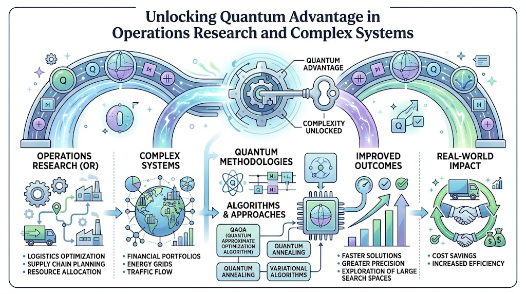
Unlocking Quantum Advantage in Operations Research and Complex Systems

Table of Contents

Introduction

Every day, global logistics networks attempt to route thousands of delivery trucks through traffic-congested cities, financial institutions balance trillions of dollars across volatile portfolios, and energy grids adjust power flow to prevent blackouts. At the core of these massive operational challenges lies a single, fundamental mathematical task: optimization. This is where quantum computing enters the conversation. By leveraging the principles of quantum mechanics—such as superposition, entanglement, and quantum interference—quantum systems explore vast solution spaces in ways classical hardware simply cannot match. Platforms like QuantumUting.com provide accessible tutorials, SDK guides, and educational frameworks designed to bridge the gap between theoretical quantum physics and practical software engineering.

What is an Optimization Problem?

At its core, an optimization problem is a mathematical challenge where the goal is to find the best possible solution among a massive set of feasible choices.

In formal terms, an optimization problem involves:

Decision Variables ($x$): The unknown choices or parameters you need to determine (e.g., whether to send a truck down Route A or Route B).
Objective Function ($f(x)$): A mathematical equation representing the goal to either minimize (e.g., cost, travel time, energy loss) or maximize (e.g., profit, throughput, efficiency).
Constraints: Rules or physical limits that valid solutions must obey (e.g., a truck cannot exceed its maximum payload weight).

$$\min_{x} f(x) \quad \text{subject to} \quad g_i(x) \le 0, \quad h_j(x) = 0$$

   +-------------------------------------------------------+
   |                 OPTIMIZATION PROBLEM                  |
   +-------------------------------------------------------+
                              |
      +-----------------------+-----------------------+
      |                                               |
      v                                               v
[ Minimize Cost / Risk ]                   [ Maximize Profit / Yield ]
      |                                               |
      +-----------------------+-----------------------+
                              |
                              v
             [ Subject to System Constraints ]

When decision variables are discrete (such as binary choices: $0$ or $1$, “yes” or “no”), the challenge becomes a combinatorial optimization problem. Examples include finding the shortest route visiting 50 cities or assigning 500 tasks to 100 servers.

Why Optimization Matters in Modern Industries

Modern industrial systems operate on tiny margins where incremental gains translate into billions of dollars in savings or revenue.

+-------------------------------------------------------------------+
|                  INDUSTRIAL OPTIMIZATION IMPACT                   |
+-------------------+-----------------------------------------------+
| Industry          | Primary Optimization Objectives               |
+-------------------+-----------------------------------------------+
| Logistics         | Fleet routing, fuel reduction, schedule delay |
| Finance           | Asset allocation, risk hedge, trade execution |
| Energy            | Grid load balance, renewable integration      |
| Manufacturing     | Job shop scheduling, supply chain bottlenecks |
+-------------------+-----------------------------------------------+

Logistics & Supply Chain: Reducing fleet mileage by just 2% saves millions of gallons of fuel and tons of carbon emissions annually.
Finance: Optimizing asset weights in an investment portfolio ensures maximum returns for a given risk threshold.
Healthcare & Pharmaceuticals: Finding the lowest energy configuration of a molecular structure accelerates drug discovery.
Telecommunications: Allocating frequency bands across cellular towers eliminates signal interference and maximizes network bandwidth.

Limitations of Classical Optimization Methods

Classical computers process information sequentially or through parallel threads using binary bits ($0$ or $1$). For simple or linear problems, classical algorithms like linear programming (Simplex algorithm) or gradient descent work exceptionally well.

However, complex real-world problems are typically non-linear and discrete, falling into the complexity class known as NP-hard or NP-complete.

    Classical Local Optima Traps vs. Global Minimum
    
    Energy / Cost
      ^
      |       /\             /\
      |      /  \   Local   /  \
      |  /\ /    \  Optimum/    \
      | /  V      \   /\  /      \
      |/           \ /  \/        \   Global Optimum
      +----------------------------\------V-------------> Solution Space

Combinatorial Explosion: As the number of variables $n$ increases, the number of possible configurations grows exponentially (often as $2^n$ or $n!$). A route with 30 cities has over $2.65 \times 10^{32}$ possible combinations.
Local Optima Traps: Traditional classical heuristics (like local search or hill climbing) get stuck in “local minima”—suboptimal solutions that look best relative to immediate neighbors, but are far from the true global optimum.
Approximation Trade-offs: To return answers in reasonable timeframes, classical solvers rely on approximation heuristics (like simulated annealing or genetic algorithms). While helpful, these methods offer no guarantee of getting close to the optimal solution as systems scale.

Introduction to Quantum Computing for Optimization

Quantum computing shifts computational paradigms by replacing classical bits with quantum bits (qubits). Rather than evaluating configurations one by one, a quantum computer manipulates a quantum state representing a superposition of all possible configurations simultaneously.

By mapping the cost function of an optimization problem into a quantum system’s energy landscape, solving the problem transforms into finding the ground state (lowest energy state) of a physical quantum system.

How Quantum Computing Approaches Optimization

Quantum computing does not rely on brute-force evaluation. Instead, it translates optimization problems into Ising Hamiltonians or Quadratic Unconstrained Binary Optimization (QUBO) models.

A general QUBO problem is expressed as:

$$f(x) = \sum_{i} q_i x_i + \sum_{i < j} q_{ij} x_i x_j, \quad x_i \in \{0, 1\}$$

When mapped to a quantum computer:

Binary decision variables ($x_i \in \{0, 1\}$) are mapped to qubit Pauli-Z operators ($\sigma_i^z \in \{+1, -1\}$).
The objective function becomes a cost Hamiltonian ($H_C$).
The lowest energy eigenstate of $H_C$ corresponds directly to the optimal solution of the original problem.

Understanding Qubits, Superposition, and Entanglement

To understand how quantum processors achieve speedups in optimization, we must look at three underlying physics principles:

+-----------------------------------------------------------------+
|                   CORE QUANTUM PRINCIPLES                       |
+-----------------------------------------------------------------+
| SUPERPOSITION    | Prepares all combinations simultaneously    |
| ENTANGLEMENT     | Correlates qubits to evaluate complex rules  |
| INTERFERENCE     | Amplifies correct paths, cancels bad paths   |
+-----------------------------------------------------------------+

1. Superposition

While a classical bit must be $0$ or $1$, a qubit can exist in a linear combination of both states until measured:

$$\vert{}\psi\rangle = \alpha \vert{}0\rangle + \beta \vert{}1\rangle$$

A register of $n$ qubits can exist in a superposition of $2^n$ computational states at once. For $n = 50$, this represents over 1 quadrillion states stored simultaneously in a single quantum wave function.

2. Entanglement

Entanglement links qubits such that the state of one qubit instantaneously dictates or correlates with the state of another, regardless of physical distance. In optimization, entanglement encodes intricate constraints between variables (e.g., “if Truck A visits City 1, Truck B cannot”).

3. Quantum Interference

Superposition creates a vast pool of possibilities; quantum interference shapes them. Quantum algorithms manipulate wave amplitudes so that paths leading to poor solutions interfere destructively (cancel out), while paths leading to optimal solutions interfere constructively (amplify).

Quantum Algorithms Used for Optimization

Several core quantum algorithms target optimization challenges, ranging from gate-based quantum circuits to special-purpose physical annealers.

                          QUANTUM OPTIMIZATION ALGORITHMS
                                         |
         +-------------------------------+-------------------------------+
         |                                                               |
  [ Variational Algorithms ]                                   [ Specialized Hardware ]
         |                                                               |
   +-----+-----+                                                         |
   |           |                                                         v
 [ QAOA ]   [ VQE ]                                             [ Quantum Annealing ]
(Gate-Based) (Chemistry/Opt)                                     (Flux Qubit Systems)

Quantum Approximate Optimization Algorithm (QAOA)

The Quantum Approximate Optimization Algorithm (QAOA), introduced by Farhi, Goldstone, and Gutmann in 2014, is a hybrid quantum-classical algorithm tailored for gate-based quantum computers running on Noisy Intermediate-Scale Quantum (NISQ) hardware.

How QAOA Works

QAOA uses alternating application of two quantum operators:

Cost Hamiltonian ($H_C$): Encodes the problem constraints and objective function.
Mixer Hamiltonian ($H_B$): Drives quantum transitions between states to explore the search space.

The parameterized quantum state is created as:

$$\vert{}\gamma, \beta\rangle = e^{-i \beta_p H_B} e^{-i \gamma_p H_C} \cdots e^{-i \beta_1 H_B} e^{-i \gamma_1 H_C} \vert{}+\rangle^{\otimes n}$$

A classical optimizer evaluates the expectation value $\langle \gamma, \beta \vert{} H_C \vert{} \gamma, \beta \rangle$ and iteratively adjusts parameters $(\boldsymbol{\gamma}, \boldsymbol{\beta})$ to minimize energy.

Quantum Annealing Explained

Quantum Annealing is a physical optimization process specifically designed for hardware like D-Wave systems. It mimics classical simulated annealing, but replaces thermal fluctuations with quantum tunneling.

    Energy Landscape & Quantum Tunneling
    
    Energy
      ^
      |      High Energy Barrier
      |           / \
      |          /   \
      |         /  *  \    <--- Quantum Tunneling passes THROUGH barrier
      |  State /   |   \        (Classical annealing must climb OVER)
      |    A  /    v    \ State B
      +------/-----------\------------------------> Configuration

Thermal Annealing: Classical particles must gain enough thermal energy to climb over high energy barriers in the solution space.
Quantum Annealing: Quantum particles can tunnel through narrow, high energy barriers, allowing the system to rapidly escape local minima and collapse into the global ground state.

Variational Quantum Algorithms (VQAs)

QAOA is a specialized instance of the broader class known as Variational Quantum Algorithms (VQAs). VQAs use shallow (low depth) parameterized quantum circuits to make the best use of today’s noisy quantum hardware. By offloading parameter optimization to classical routines, VQAs keep quantum coherence requirements low.

Hybrid Quantum-Classical Optimization

Pure quantum advantage across full enterprise workflows remains a future milestone. Today, the operational standard is Hybrid Quantum-Classical Computing.

+-------------------------------------------------------------------+
|               HYBRID QUANTUM-CLASSICAL LOOP                       |
+-------------------------------------------------------------------+
|  1. Problem Formulation (QUBO / Ising Model on Classical CPU)     |
|                             |                                     |
|                             v                                     |
|  2. Quantum Circuit Preparation (Qiskit / Gate Synthesis)         |
|                             |                                     |
|                             v                                     |
|  3. Quantum Execution (Quantum Processing Unit - QPU)             |
|                             |                                     |
|                             v                                     |
|  4. Measurement & Expectation Sampling                            |
|                             |                                     |
|                             v                                     |
|  5. Parameter Tuning (Classical Optimizer: COBYLA, SPSA, ADAM)    |
|                             |                                     |
|  +--------------------------+                                     |
|  | Loop repeats until convergence                                 |
+-------------------------------------------------------------------+

In this framework:

The Quantum Processor (QPU) handles state preparation and complex expectation sampling.
The Classical Processor (CPU/GPU) handles constraint parsing, parameter updates, and convergence checking.

Qiskit Optimization Module Overview

IBM’s Qiskit Optimization stack is an open-source framework designed for building and testing quantum optimization workflows.

Key features include:

Docplex Integration: Translates high-level mathematical models seamlessly into quantum quadratic programs.
Converter Utilities: Converts constrained problems to unconstrained QUBO formats using penalty terms automatically.
Algorithms: Native implementations of QAOA, VQE, GroverOptimizer, and GoemansWilliamsonOptimizer.

Classical vs Quantum Optimization

+---------------------------------------------------------------------------------------+
|                         CLASSICAL VS QUANTUM OPTIMIZATION                             |
+-------------------------+---------------------------------+---------------------------+
| Dimension               | Classical Optimization          | Quantum Optimization      |
+-------------------------+---------------------------------+---------------------------+
| Core Unit               | Classical Bit (0 or 1)          | Qubit (|0>, |1>, Superpos)|
| Solution Space Exploration| Sequential / Heuristic Branching| Quantum Interference &    |
|                         |                                 | Parallel Superposition    |
| Barrier Traversal       | Thermal Climbing Over Barriers  | Quantum Tunneling Through |
| Best Suited Problem Type| Convex / Smooth Continuous      | Non-Convex Combinatorial  |
| Hardware Maturity       | Highly Mature (CPLEX, Gurobi)   | NISQ / Hybrid Stage       |
| Scalability Limit       | Exponential CPU Wall for NP-Hard| Polynomial Scaling Potential|
+-------------------------+---------------------------------+---------------------------+

Industry Applications

    +---------------------------------------------------------------+
    |                  QUANTUM OPTIMIZATION USE CASES               |
    +---------------------------------------------------------------+
    | Logistics        ->  Vehicle Routing & Warehouse Allocation  |
    | Finance          ->  Portfolio Rebalancing & Arbitrage        |
    | Healthcare       ->  Molecular Docking & Protein Folding      |
    | Manufacturing    ->  Job-Shop Scheduling & Yield Planning     |
    | Energy           ->  Smart Grid Power Flow & Storage Mgmt     |
    | Telecom          ->  5G/6G Antenna Array Frequency Allocation |
    +---------------------------------------------------------------+

Logistics & Supply Chain

Vehicle Routing Problem (VRP): Optimizing delivery paths across dynamic traffic and strict delivery time windows.
Container Loading: Maximizing cargo space utilization while balancing weight distributions.

Finance & Investment

Portfolio Optimization: Selecting asset blends under discrete transaction costs and cardinality constraints.
Risk Management: Finding optimal hedging strategies across volatile derivatives markets.

Healthcare & Pharmaceuticals

Molecular Docking: Optimizing binding orientations of candidate drug molecules to target proteins.
Radiotherapy Planning: Calculating optimal radiation beam angles to target tumors while preserving healthy tissue.

Manufacturing & Telecommunications

Job-Shop Scheduling: Arranging machine sequence passes to minimize total production idle time (makespan).
Network Routing: Optimizing 5G channel allocations to minimize packet latency and cross-talk interference.

Energy & Utilities

Unit Commitment Problem: Deciding which power generators to turn on/off across varying grid demands.

Practical Examples and Sample Workflows

Below is a complete, runnable example using Qiskit Optimization to solve a standard Max-Cut combinatorial problem—a classic graph optimization challenge mapped directly to QUBO models.

Python

# Import core Qiskit and Optimization libraries
from docplex.mp.model import Model
from qiskit_optimization.algorithms import MinimumEigenOptimizer
from qiskit_optimization.translators import from_docplex_mp
from qiskit_algorithms.minimum_eigensolvers import QAOA
from qiskit_algorithms.optimizers import SPSA
from qiskit_primitives import Sampler

# Step 1: Formulate the optimization problem using Docplex
docplex_model = Model(name="MaxCut_Example")
x0 = docplex_model.binary_var(name="x0")
x1 = docplex_model.binary_var(name="x1")
x2 = docplex_model.binary_var(name="x2")

# Objective: Maximize edge cuts between connected nodes
# Cost function: (x0 - x1)^2 + (x1 - x2)^2
docplex_model.maximize(x0 + x1 + x2 - 2*x0*x1 - 2*x1*x2)

# Step 2: Convert Docplex Model to Qiskit Quadratic Program
problem = from_docplex_mp(docplex_model)

# Step 3: Initialize Classical Optimizer and Quantum Sampler Primitives
classical_optimizer = SPSA(maxiter=100)
sampler = Sampler()

# Step 4: Configure QAOA Solver
qaoa_solver = QAOA(sampler=sampler, optimizer=classical_optimizer, reps=2)
optimizer = MinimumEigenOptimizer(qaoa_solver)

# Step 5: Solve Problem
result = optimizer.solve(problem)

# Output results
print(f"Optimal Variables: {result.x}")
print(f"Optimal Objective Value: {result.fval}")

Current Hardware Limitations and Challenges

Despite massive advances, quantum computing currently faces tangible engineering challenges:

+-------------------------------------------------------------------+
|                  CURRENT NISQ HARDWARE LIMITATIONS                |
+-------------------+-----------------------------------------------+
| Challenge         | Direct Operational Impact                     |
+-------------------+-----------------------------------------------+
| Quantum Noise     | Gate errors degrade circuit output fidelity   |
| Low Qubit Count   | Limits problem variable scale (< 1,000 vars)  |
| Decoherence       | Qubits lose state before deep circuits finish |
| Limited Connectivity| Requires heavy SWAP gate overhead           |
+-------------------+-----------------------------------------------+

Noise & Decoherence: Today’s NISQ (Noisy Intermediate-Scale Quantum) systems lack fault-tolerant error correction. Qubits lose their quantum state within microseconds.
Connectivity Restrictions: Physical qubits on superconducting chips are not all connected to one another, requiring additional SWAP gates that increase circuit depth and introduce noise.
Barren Plateaus: In variational algorithms, the gradient of the parameter landscape can vanish exponentially with qubit count, making classical training difficult for large systems.

When Quantum Optimization is Appropriate

Quantum computing is not a universal replacement for classical algorithms. Determining when to use quantum optimization requires evaluating problem characteristics:

                          DECISION TREE: WHEN TO USE QUANTUM
                                         |
                       Is the problem computationally hard?
                                  /            \
                             [ Yes ]          [ No ] -> Use Classical (Gurobi / CPLEX)
                               /
             Are variables discrete or non-convex?
                            /          \
                       [ Yes ]        [ No ] -> Use Convex Classical Methods
                         /
     Can classical heuristics find optimal solutions fast enough?
                      /                 \
                [ Yes ]                 [ No ]
                  /                        \
    Use Classical Heuristics         APPLY HYBRID QUANTUM OPTIMIZATION

Use Classical Solvers When: The problem is linear, convex, or handled efficiently by mature tools like Gurobi, CPLEX, or linear programming.
Consider Hybrid Quantum Solvers When: The problem is non-convex, NP-hard, rich in discrete combinatorial choices, and classical heuristics get trapped in poor local minima.

Common Misconceptions About Quantum Computing

“Quantum computers solve everything exponentially faster.”
- Fact: Quantum speedups depend entirely on problem structure and algorithm design. Some classical algorithms remain faster for simple tasks.
“Quantum computers will render classical supercomputers obsolete.”
- Fact: Future computing infrastructure will be heterogeneous—classical CPUs/GPUs will manage data and orchestration, while QPUs act as specialized accelerators for targeted workloads.
“Quantum optimization is already outperforming classical supercomputers across enterprise tasks.”
- Fact: We are currently in the quantum utility and evaluation phase. Demonstrations show promise, but practical production quantum advantage requires larger fault-tolerant machines.

Future of Quantum Optimization

The roadmap toward universal quantum advantage follows three major technical milestones:

+-------------------------------------------------------------------+
|               QUANTUM OPTIMIZATION DEVELOPMENT ROADMAP             |
+-------------------------------------------------------------------+
|  1. NISQ Era (Present - 2028):                                    |
|     * Hybrid algorithms (QAOA, VQE)                               |
|     * Error suppression and mitigation techniques                 |
|     * Proof-of-concept enterprise pilot projects                    |
|                                                                   |
|  2. Quantum Utility Era (2028 - 2032):                            |
|     * Logical qubits backed by early error correction             |
|     * Demonstrable quantum advantage on specific sub-problems     |
|                                                                   |
|  3. Fault-Tolerant Quantum Era (2032+):                           |
|     * Millions of physical qubits forming resilient logical qubits|
|     * Provable quadratic and exponential speedups for global search |
+-------------------------------------------------------------------+

Career Opportunities in Quantum Computing

As investments in quantum technology accelerate, demand for skilled professionals is soaring:

Quantum Algorithm Engineer: Designs mathematical representations of real-world problems and maps them to quantum circuits.
Quantum Software Developer: Builds robust SDKs, converters, and cloud interfaces (e.g., using Qiskit, Cirq, or Pennylane).
Optimization Specialist / OR Analyst: Formulates complex operational models into QUBO and Ising structures.
Quantum Applications Scientist: Partners with enterprise leaders to implement domain-specific quantum workflows.

Learning Roadmap for Beginners

If you want to build practical skills in quantum optimization, follow this structured four-stage pathway:

+-------------------------------------------------------------------+
|                    BEGINNER LEARNING ROADMAP                      |
+-------------------------------------------------------------------+
|  STAGE 1: Foundational Math & Python                              |
|  * Linear Algebra (vectors, matrices, eigenvalues)                |
|  * Python proficiency (NumPy, SciPy)                              |
|                                                                   |
|  STAGE 2: Core Quantum Mechanics Principles                       |
|  * Quantum states, Dirac notation (|psi>), measurement            |
|  * Basic logic gates (Hadamard, CNOT, Pauli-Z)                    |
|                                                                   |
|  STAGE 3: Optimization Formulations                               |
|  * Graph theory basics (Max-Cut, Travelling Salesperson)          |
|  * Mathematical modeling (QUBO, Ising Hamiltonians)              |
|                                                                   |
|  STAGE 4: Hands-on SDK Implementation                             |
|  * Code workflows using Qiskit Optimization                       |
|  * Run simulations on Aer and submit jobs to real IBM Quantum hardware|
+-------------------------------------------------------------------+

Frequently Asked Questions (10 FAQs)

Q1: What is quantum optimization?

Quantum optimization is a field of quantum computing that uses quantum mechanics—specifically algorithms like QAOA and quantum annealing—to solve complex mathematical optimization problems faster or more accurately than purely classical methods.

Q2: How does QAOA differ from Quantum Annealing?

QAOA is a gate-based hybrid algorithm that runs on general-purpose quantum computers using quantum logic circuits. Quantum Annealing relies on purpose-built analog quantum hardware that naturally evolves a physical system toward its lowest energy state.

Q3: What is a QUBO model?

QUBO stands for Quadratic Unconstrained Binary Optimization. It is a standardized mathematical matrix formulation used to express combinatorial problems using binary variables ($0$ and $1$), making them directly readable by quantum solvers.

Q4: Can current quantum computers outperform classical solvers today?

For small-to-medium enterprise problems, classical solvers like Gurobi remain faster and more reliable. Today’s quantum systems are used primarily for research, benchmarking, algorithm development, and early hybrid workflows preparing for fault-tolerant hardware.

Q5: What is the NISQ era?

NISQ stands for Noisy Intermediate-Scale Quantum. It refers to the current era of quantum hardware characterized by 50 to a few thousand physical qubits that lack full error correction and are susceptible to environmental noise.

Q6: Do I need a background in quantum physics to learn quantum optimization?

No. While basic knowledge of linear algebra is helpful, modern quantum SDKs like Qiskit allow developers, data scientists, and software engineers to program quantum algorithms using Python without needing an advanced physics degree.

Q7: What software tools are best for practicing quantum optimization?

IBM’s Qiskit Optimization, D-Wave’s Ocean SDK, Google’s Cirq, and Classiq are industry-standard open-source toolkits for formulating and executing quantum optimization workflows.

Q8: What is a hybrid quantum-classical algorithm?

A hybrid algorithm combines classical and quantum processing in a closed loop. The quantum processor prepares complex states and measures expectation values, while a classical computer optimizes parameters to guide the system toward the best solution.

Q9: Why is Max-Cut frequently used as an optimization example?

Max-Cut is a classic NP-complete graph theory problem that maps cleanly onto Ising spin glasses and QUBO frameworks, making it an ideal benchmark for testing new quantum algorithms like QAOA.

Q10: How will quantum computing impact supply chain management?

Quantum computing will allow logistics networks to analyze millions of dynamic variables—such as real-time traffic, weather disruption, fleet capacity, and delivery schedules—simultaneously, reducing transit times and operational costs.

Conclusion

Quantum computing represents a fundamental shift in how humanity tackles complex operational challenges. By replacing brute-force iteration with quantum interference, superposition, and tunneling, quantum optimization opens new possibilities across logistics, finance, healthcare, and energy management. While current hardware remains in the NISQ era, hybrid quantum-classical workflows are laying the technical foundation for scalable enterprise advantage. Organizations, researchers, and developers who master quantum formulation techniques today will lead the next era of high-performance computing.