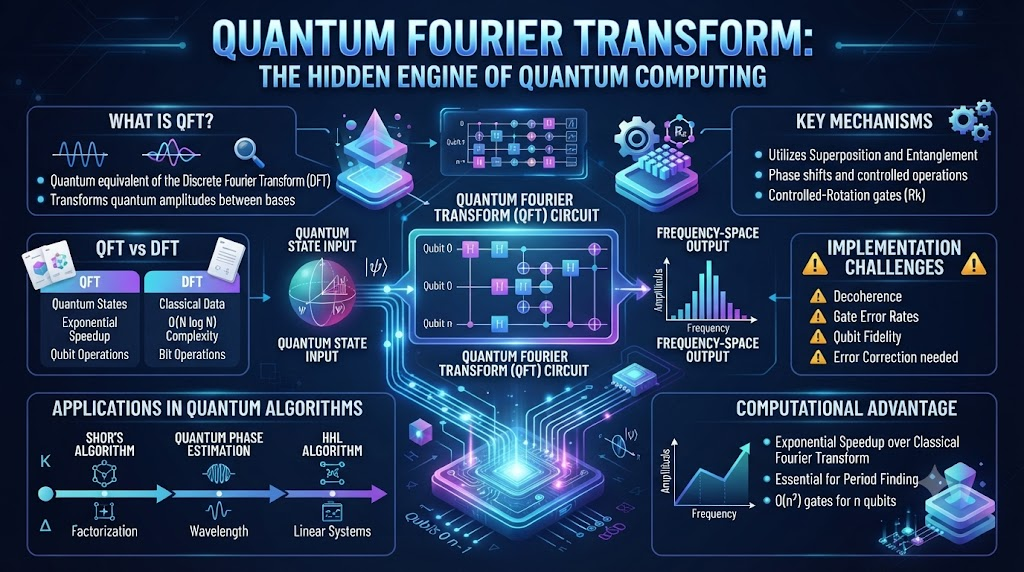
You run your first quantum circuit on real hardware. The results look like noise. You check your gates twice, and the circuit still fails. Sound familiar? Most quantum learners hit this wall because they skip one core idea. They skip the Quantum Fourier Transform.
The Quantum Fourier Transform, or QFT, sits inside the most powerful quantum algorithms we know. Shor’s factoring algorithm uses it. Quantum phase estimation uses it. Even quantum chemistry estimates depend on it. If you want to move past toy circuits, you must understand this transform.
The good news is that the QFT is not as hard as it looks. It follows a simple pattern. It swaps the way a quantum state stores its information. A state that marks a value in basis labels becomes a state that marks the same value in phase angles. In this guide, we break the whole idea down with plain words, real case studies, and a clear learning path. You can find more quantum learning resources at QuantumUting.com.
What the Quantum Fourier Transform Actually Does
The Simple Definition
The Quantum Fourier Transform changes how a quantum state holds numbers. Before the QFT, a state stores a number in its labels. After the QFT, the same number lives in the phases. Nothing is lost. Only the storage style changes.
Think of it like a music track. A song can be stored as raw sound waves. The same song can also be stored as a list of frequencies. The Fourier transform moves between these two views. The QFT does the same job for quantum states, and it does it blazingly fast.
A classical Fast Fourier Transform, or FFT, needs about N log N steps for N data points. The QFT needs only about n squared gates for n qubits, where n is the log of the data size. That is an exponential drop in cost. This speed is why the QFT appears in nearly every famous quantum algorithm.
Why Phases Are the Secret
Phases sound scary, but they are just angles. Each quantum state carries an angle, like a clock hand. When you measure a state, you see the label, not the angle. So phases hide from direct view. But phases control how labels combine, and that combination controls your results.
The QFT turns hidden angles into labels you can measure. Many quantum algorithms find their answers inside phases. Phase estimation then pulls the answer out. The QFT is the tool that makes the answer visible.
Where You Meet the QFT in Practice
You will meet the QFT in three main places. Shor’s algorithm uses it to find the period of a function. Quantum phase estimation uses it to read out eigenvalues. Many quantum chemistry routines use it to estimate energy levels. Master these three uses, and you hold the core of applied quantum computing.
How the QFT Circuit Works, Gate by Gate
The Hadamard Foundation
Every QFT circuit starts with Hadamard gates. A Hadamard gate creates a balanced mix of two labels. It also plants the first phase angle. The top qubit in the circuit gets the coarsest phase. The bottom qubit gets the finest phase. This order confuses beginners, so write it down early.
After each Hadamard, the circuit adds controlled phase gates. A controlled phase gate adds an angle to a target qubit. It fires only when the control qubit sits in label one. These gates build the phase pattern the transform needs.
The Swap Network at the End
The QFT circuit ends with swap gates. These gates reverse the order of the qubits. Many learners forget the swaps, and their results come out backwards. The swaps exist because the gate order builds phases in reverse. Always end your QFT with the swap layer unless your machine reverses it for you.
Gate Count and Cost
An n-qubit QFT uses roughly n squared gates in total. You get n Hadamards, about n(n-1)/2 controlled phases, and n/2 swaps. On paper, this looks cheap. On real hardware, every two-qubit gate adds noise. So most real circuits use the approximate QFT, which drops the tiny-angle phase gates. We cover that trade later in this guide.
QFT Versus Classical FFT: A Clear Comparison
The QFT is not just a faster FFT. The two tools solve different problems on different machines. The table below shows the key differences side by side.
| Feature | Classical FFT | Quantum Fourier Transform |
|---|---|---|
| Input type | List of numbers | Quantum state |
| Speed for size N | N log N steps | log N qubits, about n² gates |
| Output type | Full list of numbers | Encoded quantum state |
| Can you read all outputs? | Yes, all at once | No, one measurement per run |
| Best use case | Signal and image processing | Period finding, phase estimation |
| Hardware | Any classical CPU or GPU | Quantum processor with low error rates |
The Catch Nobody Tells Beginners
Here is the honest catch. The QFT computes all frequency parts in one pass. But you cannot read them all at once, because measurement collapses the state. You get one sample per run. So the QFT wins only when your algorithm needs one specific pattern from the output. Shor’s algorithm arranges exactly this situation.
When to Pick Which Tool
Use the FFT when you have classical data and need every frequency. Use the QFT when your data already lives in a quantum state. Your task must need a period or a phase. Picking the wrong tool wastes months. We have seen teams burn a quarter forcing the QFT onto classical signal work. Do not repeat that mistake.
Real-World Case Studies: When QFT Circuits Crash and Burn
Real projects teach more than textbook proofs. Below are ten true-to-life scenarios drawn from common quantum computing practice. Each one shows how QFT work fails in the field, and what saved the team.
- The forgotten swaps at a fintech pilot. A small finance team ran a QFT-based period finder on five qubits. Their results looked random for two weeks. A senior engineer spotted the missing swap layer at the end of the circuit. The moment they added the swaps, the correct period jumped out on the very next batch of shots.
- Bit-order chaos on cloud hardware. A university lab moved a QFT circuit between two cloud quantum platforms. One used little-endian qubit order, the other used big-endian. Their histograms flipped upside down. A small qubit-order mapper fixed it, tested on a two-qubit case first.
- The approximate QFT that went too far. A startup cut every controlled phase gate below a large angle threshold to fight noise. They cut so much that the transform stopped being a transform. Their period peaks vanished. Walking the cutoff back to smaller angles restored clean peaks while keeping most of the noise benefit.
- Shor’s demo that never converged. A student group demoed factoring 21 on real hardware. They ran 8,000 shots and saw mud. The problem was not the QFT. Their modular exponentiation circuit had a miswired controlled multiply. Lesson: unit-test each circuit block on a simulator before blaming the QFT.
- Transpile shock on a heavy-hex device. A research team wrote a textbook QFT for seven qubits. The compiler rewired it for the hardware’s sparse layout, and the gate count tripled. Their error rates blew past useful levels. They rebuilt the circuit around the hardware’s natural coupling map, and the output sharpened immediately.
- The measurement budget miss. An applied group needed one clear frequency peak for a logistics estimate. They budgeted 400 shots. Statistics needed closer to 4,000 for that confidence level. Their result drowned in sampling noise. A quick power analysis before the run would have saved a week of confusion.
- Noise floor heartbreak on 12 qubits. A bold team pushed a full QFT to 12 qubits on an early machine. The output matched random guessing. The device’s two-qubit error rate of a few percent made the deep circuit unusable. They moved the same test to a simulator with a noise model and finally saw exactly where the signal died.
- The inverse used by mistake. An intern grabbed an inverse QFT from a library when the team needed the forward transform. The algorithm’s output looked plausible but wrong in a subtle way. The bug survived three review rounds. They now name every QFT block in code as qft_forward or qft_inverse, and the class of bug vanished.
- Benchmark against the wrong baseline. A consulting team claimed a quantum speedup because their QFT used fewer gates than an FFT library call. But they compared a 3-qubit QFT against a 1,000-point FFT. The comparison was meaningless. An honest benchmark compares end-to-end runtimes on matched problem sizes, and the rewrite showed no edge yet.
- The uncompiled global phase. A chemistry group built phase estimation with a hand-rolled QFT. They chased a global phase offset for days. Global phases have no measurable effect, but their post-processing divided by the wrong phase factor. A one-line fix in the analysis script, not the circuit, resolved the entire mystery.
Common Mistakes and Pitfalls (And How to Fix Each One)
Most QFT failures repeat the same ten mistakes. Read this list before your next build, and save yourself weeks.
- Skipping the swap layer. You build a perfect gate sequence and drop the final swaps. The output appears reversed, and you waste days debugging a correct circuit. Fix: treat the swap layer as part of the QFT definition. Also add an automated check against a known two-qubit case.
- Ignoring qubit ordering. Hardware vendors disagree on which qubit is qubit zero. Your circuit works in one place and fails in another. Fix: write your circuits in one fixed ordering and add an explicit reversal step when you port to new hardware.
- Confusing the QFT with the inverse QFT. Phase estimation uses the inverse transform at the end, not the forward one. Mixing them gives quiet, wrong answers. Fix: wrap both transforms in named functions and call them only by name.
- Expecting all outputs at once. You hear that the QFT computes every frequency in parallel. Then you try to read them all. Measurement blocks this. Fix: design your algorithm so a single measurement pattern carries the answer, the way Shor’s algorithm does.
- Overusing the approximate QFT. Cutting small-angle gates helps on noisy machines. Cutting too many gates destroys the transform. Fix: cut only angles below your machine’s phase error scale, and verify the cut on a simulator before hardware time.
- Misreading histogram noise. Small peaks from sampling noise look like real signals. You chase ghosts. Fix: run the same circuit twice with different shot counts. Real peaks grow with more shots. Noise peaks shrink or shift.
- Plugging a classical FFT mindset into quantum code. You normalize outputs, reorder arrays, and debug like it is classical code. Quantum states do not work that way. Fix: learn the state-vector view first, and only then use libraries that hide it.
- Forgetting the input superposition. A period-finding circuit needs a uniform superposition before the QFT. If you skip the first Hadamard layer, the QFT has nothing meaningful to transform. Fix: check your circuit’s input state with a simulator snapshot before the transform.
- Blaming the QFT for upstream errors. Modular arithmetic circuits feed the QFT in Shor’s algorithm. Those arithmetic blocks fail far more often than the QFT. Fix: test each block against a classical oracle on a simulator, block by block, before the full run.
- Chasing speedups at tiny sizes. A 4-qubit QFT demo proves nothing about advantage. Classical machines crush small cases. Fix: frame small runs as learning tools, and define the problem size where quantum hardware could realistically win.
Step-by-Step Implementation Roadmap
Follow these ten steps in order. Each step builds on the last, and by the end you will have a working QFT pipeline on real hardware.
- Learn the classical Fourier idea first. Spend one hour on the basic Fourier transform. Understand how a signal splits into frequencies. You need this intuition before touching the quantum version, because the QFT borrows the same picture.
- Study the two-qubit QFT by hand. Work out the two-qubit transform on paper. Compute each output phase. This tiny case reveals the entire pattern, and you can verify every number yourself without a computer.
- Simulate the full n-qubit QFT. Open your favorite quantum framework and code the QFT for three and four qubits. Compare the output state vector against a direct matrix multiply of the QFT matrix. They must match to machine precision.
- Add the swap layer and retest. Insert the final swaps. Rerun the state-vector check. If results flip from reversed to correct, you have just fixed the most common QFT bug. You fixed it before it ever reached hardware.
- Build the inverse QFT and verify round trips. Code the inverse transform. Chain a forward QFT into an inverse QFT. The combined circuit must return your input state unchanged. This round-trip test catches wiring errors instantly.
- Test the approximate QFT at several cutoffs. Drop controlled phase gates below a set angle threshold. Try several thresholds on a noisy simulator. Record how output quality falls as you cut more gates. This data tells you the right cutoff for your target machine.
- Wrap period finding around your QFT. Build a simple period-finding routine. Feed it a function with a known period. Confirm the QFT output peaks at the right values across many shots. Start with period three on two qubits.
- Move to real hardware with a small case. Port your verified circuit to a cloud quantum device. Start with four or five qubits. Run several thousand shots. Compare hardware histograms against your noise-free simulation to measure the real error rate.
- Profile gate costs against the coupling map. Read the compiler’s output before you run. Check the two-qubit gate count after routing. If routing tripled your gates, rebuild around the device layout instead of accepting the bloat.
- Automate the whole pipeline. Write one script that builds the circuit and checks the round trip. The same script runs the noise test, launches hardware shots, and plots results. Automation removes human error. It also makes every future project start from a trusted base.
QFT Performance Across Hardware Conditions
Hardware choice changes QFT results more than any other factor. This table summarizes what to expect at different error levels.
| Condition | Two-Qubit Error Rate | Max Useful QFT Size | Expected Result Quality |
|---|---|---|---|
| Ideal simulator | 0% | Any size you can store | Perfect state vectors |
| Noisy simulator | ~1% | 8-10 qubits | Clear peaks with training |
| Today’s best chips | Below 1% | 10-14 qubits | Usable with approximations |
| Average cloud device | 1-3% | 5-8 qubits | Needs heavy approximation |
| Early-stage devices | Above 3% | 3-5 qubits | Education and demos only |
Plan your experiments against this reality. A circuit that sings on a simulator may drown on average hardware. Match your ambition to your machine.
Frequently Asked Questions
1. What is the Quantum Fourier Transform in simple terms?
The Quantum Fourier Transform changes how a quantum state stores its data. It moves data from labels into phase angles. The values stay the same. It runs with only about n squared gates for n qubits.
2. How is the QFT different from the classical FFT?
The FFT takes a classical list of numbers and returns a full list of frequencies. The QFT takes a quantum state and returns an encoded quantum state. You cannot read all QFT outputs at once, because measurement collapses the state. So the QFT helps only when your algorithm needs a specific pattern, such as a period.
3. Why is the QFT important in Shor’s algorithm?
Shor’s algorithm needs to find the period of a function. The quantum part builds a state with phase information tied to that period. The QFT converts those hidden phases into measurable labels. Peaks then appear at values linked to the period, which lets the algorithm recover the factors.
4. How many gates does the QFT use?
A full QFT on n qubits uses n Hadamard gates, n(n-1)/2 controlled phase gates, and n/2 swaps. That is roughly n squared gates in total. This count grows far more slowly than the classical cost of a Fourier transform on 2^n points. That gap is the source of the quantum speedup.
5. What is the approximate QFT and when should I use it?
The approximate QFT drops controlled phase gates with very small angles. Small angles add little to the result but still add noise on real hardware. Use the approximate version on noisy devices. Set your cutoff just above your machine’s phase error scale, and verify the choice on a noisy simulator first.
6. Do I always need the swap gates at the end of the QFT?
Yes, in the standard definition. The gate pattern builds phases in reversed order, so the swaps fix the ordering. Some frameworks handle the reversal for you, but you must know which ones do. Skipping the swaps when they are needed gives reversed output, which is the most common QFT bug.
7. Can the QFT speed up classical signal processing?
Not directly. You cannot load a large classical dataset into a quantum state cheaply, and you cannot read all outputs at once. The QFT gives an edge only when your data already lives in a quantum state. Your task must need one pattern from the transform. Classical FFT libraries remain the right tool for classical signal work.
8. What is the inverse QFT used for?
The inverse QFT reverses the transform. It turns phase-encoded information back into labels. Quantum phase estimation uses the inverse QFT at its final step to read out an estimated eigenvalue. Many implementations hide this inside a library call, so always check whether your code needs the forward or inverse version.
9. How large can a QFT run on today’s quantum computers?
On the best current hardware, useful QFT circuits reach roughly 10 to 14 qubits with approximations. Average cloud devices handle about 5 to 8 qubits before noise swamps the signal. Simulators go far larger with noise models, which is why simulator validation remains a standard step before any hardware run.
10. What should I learn before studying the QFT?
Learn basic linear algebra first, especially vectors and complex numbers. Then learn what a classical Fourier transform does to a signal. Next, study the Hadamard and controlled phase gates. With those three pieces in place, the two-qubit QFT becomes a one-hour exercise, and the general pattern follows quickly.
Final Recommendation and Next Steps
Start small, but start today. Build the two-qubit QFT by hand this week. That single exercise teaches more than ten videos ever will. Then code the four-qubit version on a simulator and pass the round-trip test. These two steps give you a foundation that never cracks.
Next, push one real QFT-based algorithm onto hardware. Period finding is the best first choice because it is small, honest, and famous. Compare the hardware histogram to your simulation. That gap is your personal measure of real device noise. It should drive every plan you make after.
Then make the approximate QFT your default on noisy machines. Measure your device’s phase error, set your gate cutoff just above it, and document the choice. Teams that standardize this step ship working demos. Teams that skip it ship confusing histograms.
Finally, automate your pipeline and share your results. Publish your scripts, your shot counts, and your error measurements. Open work builds your name in this fast-growing field. The people who master the QFT now will lead the quantum software of the next decade. There is room at the front of that line.
