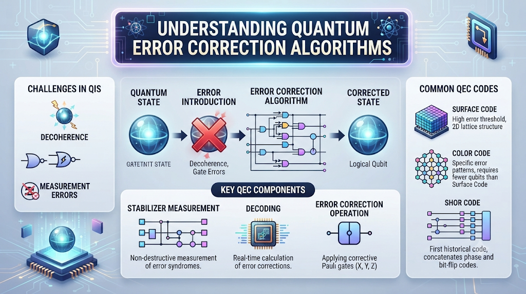
Building fault-tolerant quantum computers is one of the most formidable engineering challenges in modern physics. Unlike classical bits, which are robust and easily protected using simple redundancy like repetition codes, quantum bits (qubits) are inherently fragile. They suffer from continuous decoherence caused by environmental noise, gate imperfections, and thermal fluctuations. Furthermore, the no-cloning theorem prevents us from simply copying an unknown quantum state to back it up. Understanding quantum error correction algorithms is essential for bridging the gap between noisy intermediate-scale quantum (NISQ) devices and large-scale, fault-tolerant quantum processors.

The Fundamental Vulnerability of Qubits

Classical error correction relies on discrete bit flips where a state is definitively 0 or 1. In contrast, qubits exist in continuous superposition states and can experience both bit-flip ($X$) errors and phase-flip ($Z$) errors, as well as continuous rotations along the Bloch sphere.

Why Classical Error Correction Fails in Quantum Systems

• Continuous Error Spectra: Quantum errors are analog in nature; a stray magnetic field can induce a tiny, continuous phase rotation rather than a clean discrete flip.
• The No-Cloning Theorem: We cannot duplicate an arbitrary quantum state to check for discrepancies without destroying the superposition.
• Measurement Collapse: Measuring a qubit directly to check its state collapses the wave function, destroying the computation in progress.

To solve this, quantum error correction (QEC) encodes a single logical qubit into a entangled state of multiple physical qubits, allowing syndrome measurements to detect errors without revealing or destroying the underlying quantum information.

Core Principles of Quantum Error Correction

Quantum error correction algorithms operate by mapping fragile logical states into a subspace of a larger multi-qubit Hilbert space.

1. Syndrome Extraction and Error Detection

Instead of measuring the data qubits directly, stabilizer measurements are performed using ancillary qubits. These measurements yield error syndromes—discrete feedback signals that indicate what error occurred and where, without providing any information about the actual computational state being processed.

2. Discretization of Errors

A remarkable feature of quantum error correction is the discretization of errors. Even though physical errors are continuous, when syndrome measurements project the state back into the code space, the continuous noise is mapped onto a discrete set of Pauli operators ($I, X, Y, Z$). This allows the quantum processor to apply precise corrective corrections.

Practical Implementation: The Steane $[7,1,3]$ Code Workflow

To understand how QEC works in practice, consider the Steane code, a CSS (Calderbank-Shor-Steane) code that encodes 1 logical qubit into 7 physical qubits and can correct an arbitrary single-qubit error (bit-flip, phase-flip, or both).

[Logical State |psi> ] ──> [ Encoding Circuit (7 Physical Qubits) ]
                                          │
                                          ▼
                             [ Noisy QPU Environment (NISQ) ]
                                          │
                                          ▼
                             [ Ancillary Syndrome Measurement ]
                                          │
                                          ▼
                             [ Classical Decoder (Lookup / MWPM) ]
                                          │
                                          ▼
                             [ Corrective Pauli Gate Applied ]

Step-by-Step Execution Workflow

1. State Encoding: Prepare a logical zero or one by entangling 7 physical data qubits using a network of Hadamard and CNOT gates.
2. Circuit Execution & Noise Injection: Run the quantum circuit steps while environmental decoherence and gate infidelities introduce errors into the physical qubits.
3. Syndrome Measurement: Introduce ancillary qubits and apply multi-qubit parity check gates corresponding to the stabilizer generators of the Steane code.
4. Classical Decoding: Read out the ancillary measurement results (syndrome bits) and pass them to a classical decoder algorithm (such as Minimum Weight Perfect Matching) to identify the error location.
5. Active Correction: Apply a targeted Pauli correction gate ($X$, $Z$, or $Y$) to the affected physical qubit to restore it to the code subspace.

Decision Guidance: Benefits, Limitations, and Alternatives

Implementing quantum error correction requires navigating severe physical resource overheads. Teams must evaluate whether their hardware maturity justifies the approach.

Advantages

• Fault-Tolerant Scaling: Enables arbitrarily long quantum computations by suppressing logical error rates below physical error rates.
• Protection Against Decoherence: Actively counters phase and bit-flip errors before they accumulate and corrupt the entire computation.
• Algorithmic Reliability: Essential for running deep quantum algorithms like Shor’s algorithm or large-scale molecular simulations.

Limitations and Constraints

• Massive Overhead: Fault-tolerant quantum computation requires thousands to millions of physical qubits to sustain a single logical qubit due to the footprint of error correction circuits.
• Latency Bottleneck: Syndrome extraction and classical decoding must happen in real time between gate cycles, imposing strict speed constraints on the control hardware.
• Overhead of Fault-Tolerant Gates: Implementing logical gates fault-tolerantly (via magic state distillation or transversal gates) significantly increases circuit depth and resource requirements.

When NOT to Use Full QEC

• NISQ-Era Variational Algorithms: If you are executing shallow quantum circuits (like VQE or QAOA) on current noisy hardware, implementing full QEC overhead will likely introduce more errors than it fixes due to the sheer volume of additional entangling gates required for syndrome extraction.

Risks and Failure Modes

Failing to account for the operational realities of QEC can lead to catastrophic error propagation rather than error suppression.

• Fault-Tolerant Violations: If error correction circuits themselves are not fault-tolerant, a single faulty ancillary qubit can spread errors across multiple data qubits, worsening the overall state fidelity.
• Decoding Latency Bottlenecks: If classical decoders cannot process syndrome measurements faster than the decoherence time of the physical qubits, the system suffers from uncorrected error buildup.
• Crosstalk Amplification: Adding numerous control lines and ancilla measurement cycles for QEC can increase physical cross-talk between neighboring qubits.

Verification and Success Metrics

To verify that your quantum error correction scheme is functioning correctly, track quantitative performance metrics:

• Logical Error Rate ($P_L$): Measure whether the error rate of the encoded logical qubit decreases as the physical error rate ($p$) drops below the fault-tolerance threshold ($p < p_{th}$).
• Threshold Verification: Compare performance across different code distances (e.g., distance-3 vs. distance-5 surface codes) to confirm that larger codes yield lower logical failure rates.
• Syndrome Extraction Fidelity: Track the operational fidelity of ancilla initialization, entangling, and measurement cycles.

Frequently Asked Questions

Q1. What is the primary purpose of quantum error correction algorithms? Quantum error correction algorithms protect fragile quantum information from environmental decoherence and gate errors by encoding logical qubits across multiple entangled physical qubits.

Q2. Why can’t we simply copy a qubit to protect it against errors? The no-cloning theorem of quantum mechanics proves that it is impossible to create an identical copy of an unknown arbitrary quantum state without destroying the original.

Q3. What is the difference between bit-flip and phase-flip errors? A bit-flip error interchanges the computational basis states $\vert{}0\rangle$ and $\vert{}1\rangle$ (analogous to a classical NOT gate), whereas a phase-flip error alters the relative sign between the superposition amplitudes.

Q4. What is the physical overhead required for fault-tolerant quantum computing? Practical fault-tolerant quantum computation requires a high overhead, where thousands to millions of physical qubits are bundled together to form a single stable logical qubit protected by error-correcting codes.

Q5. How do quantum error correction codes detect errors without measuring the data? Algorithms use stabilizer measurements involving ancillary qubits to check parity traits of the system, revealing error syndromes without collapsing the superposition of the protected data.

Q6. What is the surface code, and why is it popular? The surface code is a prominent topological quantum error correction code arranged on a 2D grid, prized because it only requires nearest-neighbor physical qubit interactions, making it highly feasible for superconducting architectures.

Q7. What role does classical computing play in quantum error correction? Classical computers must process real-time syndrome measurement outputs, run decoding algorithms to identify error locations, and issue corrective commands within strict timing windows before the next gate cycle.

Q8. What is the fault-tolerance threshold? The fault-tolerance threshold is the maximum physical error rate per gate below which adding more physical qubits to an error-correcting code successfully reduces the overall logical error rate.

Q9. Can current NISQ computers run full quantum error correction? Current NISQ devices lack the scale and low physical error rates required to run fault-tolerant QEC with a net benefit, though they routinely run smaller error-mitigation and error-detection experiments.

Q10. How do magic state distillation protocols assist QEC? Magic state distillation is a resource-intensive procedure used to prepare clean, high-fidelity non-Clifford states required for universal fault-tolerant quantum computation, overcoming the limitations of standard transversal gates.

Conclusion

Understanding quantum error correction algorithms reveals the mathematical and architectural backbone required to scale quantum computers beyond noisy intermediate limitations. By mastering stabilizer codes, syndrome extraction, and fault-tolerant decoding, researchers pave the way for stable, scalable quantum architectures. Review your hardware topology constraints and begin modeling small-scale error-correcting codes in simulation frameworks today.